Vary volume fraction of the two species
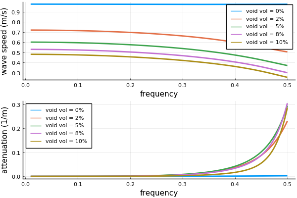
Here we demonstrate how varying the volume fraction of two different species of particles changes the effective wave speed and attenuation.
Define the material
using EffectiveWaves

# for fixed total volume fraction
background = Acoustic(3; ρ = 1.0, c = 1.0) # 3 for a 3D material.


gas_particle = Particle(Acoustic(3; ρ = 0.3, c = 0.3), 0.5) # 0.5 is the radius
solid_particle = Particle(Acoustic(3; ρ = 1000.0, c = 1000.0), 1.5)
Calculate how the wavenumbers change when varying the volume fractions
ωs = LinRange(0.01,0.5,200)

N=5
volumefraction = 0.1
vols = LinRange(0.0,volumefraction,N)

ks_arr = map(1:N) do i
    sp1 = Specie(gas_particle; volume_fraction = vols[i])
    sp2 = Specie(solid_particle; volume_fraction = volumefraction-vols[i])
    [ wavenumber_low_volumefraction(ω, background, [sp1,sp2]) for ω in ωs]
end

speeds = [ ωs ./ real(ks) for ks in ks_arr]
attenuations = imag.(ks_arr)
Plot the results
labs = reshape( map(v -> "void vol = $(Int(round(100*v)))%",vols),1, length(vols));
p1 = plot(ωs, speeds,
    labels=labs,
    ylabel="wave speed (m/s)" ,xlabel="frequency"
);
p2 = plot(ωs, attenuations,
    labels=labs, xlabel="frequency", ylabel="attenuation (1/m)");
plot(p1,p2,layout=(2,1))