Simple random particles example

## Define particle properties
Define the volume fraction of particles, the region to place the particles, and their radius

julia using MultipleScattering num_particles = 4 radius = 1.0

particlemedium = Acoustic(2; ρ=0.2, c=0.1) # 2D particle with density ρ = 0.2 and soundspeed c = 0.1 particleshape = Circle(radius)

maxwidth = 20*radius bottomleft = [0.,-maxwidth] topright = [maxwidth,maxwidth] region_shape = Box([bottomleft,topright])

particles = randomparticles(particlemedium, particleshape; regionshape = regionshape, numparticles = num_particles)

Now choose the receiver position `x`, the host medium, set plane wave as a source wave, and choose the angular frequency range `ωs`

julia x = [-10.,0.] hostmedium = Acoustic(2; ρ=1.0, c=1.0) source = planesource(host_medium; position = x, direction = [1.0,0.])

ωs = LinRange(0.01,1.0,100)

simulation = FrequencySimulation(particles, source) result = run(simulation, x, ωs)

We use the `Plots` package to plot both the response at the listener position x

julia using Plots; #pyplot(linewidth = 2.0) plot(result, fieldapply=real) # plot result plot!(result, fieldapply=imag) #savefig("plot_result.png")

![Plot of response against wavenumber](plot_result.png)

And plot the whole field inside the region_shape `bounds` for a specific wavenumber (`ω=0.8`)

julia bottomleft = [-15.,-maxwidth] topright = [maxwidth,max_width] bounds = Box([bottomleft,topright])

#plot(simulation,0.8; res=80, bounds=bounds)
#plot!(region_shape, linecolor=:red)
#plot!(simulation)
#scatter!([x[1]],[x[2]], lab="receiver")

#savefig("plot_field.png")

```

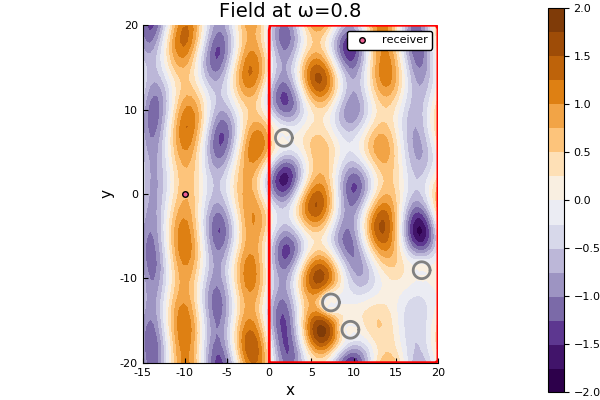
Things to try

• Try changing the volume fraction, particle radius and ω values we evaluate